The Hidden Cost of VertiPaq Scans

One of the most rewarding parts of working with DAX is discovering that two measures can return exactly the same result while taking very different paths through the engine.

To the report user, there is no difference. The number is correct, the visual renders, and the report appears to work.

But behind the scenes, one version may be asking VertiPaq to do far more work than necessary.

On a small model, that difference might be measured in milliseconds. On a large enterprise model with hundreds of millions of rows, repeated measure evaluations across visuals, slicers, and report interactions can turn those milliseconds into a real performance and capacity problem.

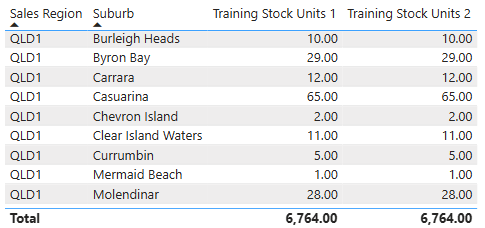
Recently, I was reviewing a measure designed to identify training stock units—products that had units recorded but no associated sales. The original measure worked correctly, but a small rewrite reduced the execution time from 14 ms to 7 ms and cut the number of Storage Engine queries from five to two.

While 7 milliseconds might not seem significant in isolation, these optimisations compound quickly in enterprise Power BI models where a measure can be evaluated thousands of times across visuals, slicers, and report interactions.

Let’s look at what changed and why it matters.

---

The Goal

The measure needed to calculate the total number of training stock units sent to clients for specific product categories.  A transaction was identified as training stock if it had a $0 sales value.  A simple enough proposition, but the catch was that there were a handful of special bundle deals where product could have $0 value but was not considered training stock.

So, to determine the total units of training stock required the construction of a virtual DAX table at run time to identify the correct training stock products, and it was the way this virtual table was handled during evaluation that made all the difference in the performance.

---

The Original Approach

The first version of the measure followed a familiar pattern:

At first glance, this is perfectly valid DAX:

1. Build a grouped table using SUMMARIZE.
2. Add calculated columns with ADDCOLUMNS.
3. Filter the resulting table.
4. Use CALCULATE to re-evaluate [Units] within the filtered context.

The logic is sound and returns the correct result.

The problem is how much work the engine needs to perform to get there.

---

What’s Happening Behind the Scenes?

In both cases, the FILTERed table that is being generated contains the same specific subset of data for the Total Units to be evaluated from.

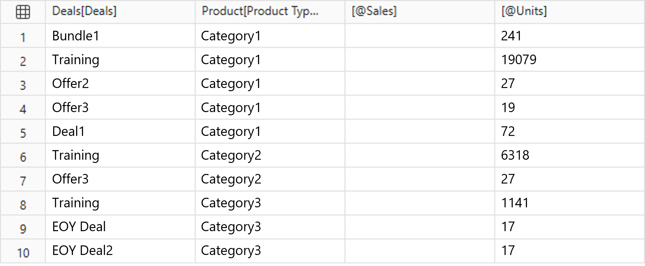
The expensive part of the calculation is here:

ADDCOLUMNS takes a table input as its first parameter, and then allows additional calculated columns to be evaluated and added to the table.  But because we are using SUMMARIZE to create the table parameter for the calculated columns to be added to, for each row in the table produced by SUMMARIZE, ADDCOLUMNS introduces a row context. Because [Sales] and [Units] are measures, each measure evaluation requires context transition so that the current row of the virtual table becomes filter context.

In other words, for every row generated by SUMMARIZE, the DAX engine must:

• Create a row context.
• Perform a context transition.
• Evaluate [Sales].
• Perform another context transition.
• Evaluate [Units].

Once the table is filtered, CALCULATE then re-evaluates [Units] once again in the new filter context.

In other words, there is a lot of Formula Engine work occurring that isn’t strictly necessary.

---

The Refactored Version

The rewritten measure uses SUMMARIZECOLUMNS instead:

Conceptually, the logic is identical:

1. Build a grouped table.
2. Filter qualifying rows.
3. Sum the resulting units.

But the execution plan is significantly different.

---

Why SUMMARIZECOLUMNS Performs Better

SUMMARIZECOLUMNS is designed to produce grouped result sets with expressions evaluated at the grouping grain. It is also the function Power BI commonly uses when generating queries for visuals, which means the engine has been heavily optimised for this pattern.

In the original measure, the engine first builds a grouped table, then iterates that table to add [Sales] and [Units], then filters the virtual table, and finally asks CALCULATE to evaluate [Units] again over the resulting filter context.

The rewritten measure changes the shape of the problem. The grouped columns and the expressions are defined together:

• group by deal and product type
• evaluate sales and units at that grain
• keep only the qualifying rows
• sum the already-calculated unit values

That is why the Storage Engine activity drops from five queries to two in this example. The improvement is not because SUMMARIZECOLUMNS is magically faster in every situation. It is because this version asks the engine a simpler question.

Rather than:

Group Rows → Add columns → Context transition → Filter → Recalculate measure

the engine can often execute:

Group Rows and Aggregate → Filter → Sum results

with far less Formula Engine involvement.

This allows more work to be pushed directly into the Storage Engine, which is where Power BI performs best.

Advantage: Better query plan and fewer formula engine operations.

As a rule of thumb:

Pattern	Typical Use
SUMMARIZE	Simple grouping, especially without measures
SUMMARIZE + ADDCOLUMNS	Group first, then add measure values in a controlled way
SUMMARIZECOLUMNS	Often a strong option when grouping and evaluating measures together

The key point is not that SUMMARIZECOLUMNS is always faster. It is that, in this scenario, it allowed the engine to produce the grouped result with fewer Storage Engine requests and less Formula Engine orchestration.

To learn more about how the SUMMARIZECOLUMNS function works, I recommend reading through SQLBI’s article on SUMMARIZECOLUMNS Best Practices.

---

The DAX Studio Evidence

One of the reasons this issue often goes unnoticed is that both versions “feel” equally fast during development.

This is why tools like DAX Studio are invaluable.

DAX Studio allows you to inspect:

• Storage Engine queries
• Formula Engine time
• Query plans
• Server timings
• VertiPaq activity

Without these metrics, optimization becomes guesswork.

With them, you can objectively compare alternatives and identify exactly where your measure is consuming resources.

If you are new to DAX Studio, I recommend taking a look at our DAX Studio for Power BI: Getting Started.

The differences between our two versions of the Training Stock Units become obvious when viewed in DAX Studio.

Original Measure

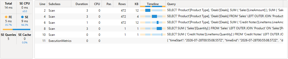
• Total Duration: 14 ms
• Formula Engine: 5 ms
• Storage Engine: 9 ms
• SE Queries: 5

The query plan shows multiple scans being generated to evaluate the grouped table and associated measures.

Refactored Measure

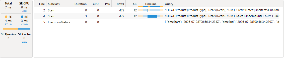
• Total Duration: 7 ms
• Formula Engine: 4 ms
• Storage Engine: 3 ms
• SE Queries: 2

The engine achieves the same result with fewer Storage Engine queries and less Storage Engine activity.

The most striking improvement is not the 7 ms reduction, but the drop from five Storage Engine queries to two. Fewer scans generally means fewer opportunities for bottlenecks as data volumes grow.

---

Why Fewer Scans Matter

Many developers focus on the DAX code itself:

SUM()
CALCULATE()
FILTER()
SUMX()

But VertiPaq does not execute DAX directly.

The Formula Engine translates DAX into Storage Engine requests. Those requests ultimately determine how much work the database performs.

Each additional Storage Engine request can mean:

• More CPU activity
• More memory access
• More query coordination
• Higher capacity consumption during report interaction
• Longer visual rendering times

On a model with only a few thousand rows, the difference might be imperceptible.

On a model with:

• 50 million transaction rows
• Multiple fact tables
• Complex matrix visuals
• Hundreds of concurrent users

those extra scans can quickly become expensive.

---

A More Readable Pattern

Performance wasn’t the only improvement.

The original calculation hides its intent inside a large CALCULATE statement:

CALCULATE (
   [Units],
FILTER (…)
)

The revised version separates each step:

VAR TrainingStockGroups =
   FILTER (…)
VAR TrainingStock =
   SUMX(…)
RETURN
   TrainingStock

This follows a pattern that is much easier to understand:

Build Table → Filter Table → Aggregate Result

When revisiting the measure six months later—or when another developer inherits the model—the logic is immediately obvious.

---

An Often Overlooked Behavioural Difference

The rewritten measure also makes the evaluation grain more explicit. The value of [Units] is calculated at the deal and product-type grain inside SUMMARIZECOLUMNS, and then those grouped values are added together with SUMX.

That can be easier to reason about because the intermediate table shows exactly what is being summed.

However, this is also something to test carefully. If [Units] later becomes a non-additive measure — for example, if it uses HASONEVALUE, DISTINCTCOUNT, AVERAGE, semi-additive time logic, or conditional logic  — then summing pre-calculated group values may not be equivalent to evaluating [Units] once in the final filter context.

In this case, because [Units] is an additive unit measure, the grouped-and-summed approach is appropriate.

---

Key Takeaways

When optimising DAX, success is rarely about finding a magical function. Instead, it comes from understanding how much work you’re asking the engine to perform.

In this case, moving from:

SUMMARIZE + ADDCOLUMNS + FILTER + CALCULATE

to:

SUMMARIZECOLUMNS + FILTER + SUMX

delivered:

• A 50% reduction in execution time (14 ms → 7 ms)
• Fewer Storage Engine queries (5 → 2)
• Reduced Formula Engine workload (removed unnecessary context transitions)
• Simpler and more maintainable code
• More predictable evaluation behaviour
• Avoids the SUMMARIZE + ADDCOLUMNS + FILTER anti-pattern.

The lesson is simple:

The biggest DAX performance gains do not always come from clever formulas. They often come from asking the engine a simpler question.

Every Storage Engine request has a cost. Individually, that cost may be tiny. Repeated hundreds or thousands of times across visuals, slicers, and report interactions, the impact can become significant.

If your goal is to build a grouped table and aggregate measure results at that grain, SUMMARIZECOLUMNS is often a strong starting point. Just do not optimise based on theory alone.

Open DAX Studio, capture Server Timings, inspect the query plan, and measure the result. The engine will tell you very quickly whether your cleaner DAX is actually faster — or whether it is just different.

Remember:

Good DAX returns the correct answer.

Great DAX returns the correct answer while asking VertiPaq to do the minimum amount of work possible.