Combine Excel Workbooks with Power Query – Method 2

Edit: Feb 2017.  Microsoft has released an update that solves the problem described in this article.  This article still has learning value however you should also take a look at the announcement from Microsoft here https://blogs.office.com/2017/02/08/january-2017-updates-for-get-transform-in-excel-2016-and-the-power-query-add-in/

There are many ways to combine data from multiple files into a single file/table in Excel.  In my first article in this series a few weeks ago, I described how to use a function to combine data from identical Excel Workbooks into a single file using Power Query.  Then last week I showed how to combine multiple CSV files into a single workbook/table using the “import from folder” method.  This week I will cover the second method to combine Excel Workbooks together.

Combining Excel files using the Folder Method

The process is essentially the same as covered last week with the CSV method with one difference covered below.

I am combining the same data as last week, but this time the file format is XLSX and not CSV.  Of course this is just test data and the process will work for 3 or 300 files.

Follow the same process as with CSV from last week

1. 1. Place all the XLSX (or other format) files in a folder
   2. Import the contents of the folder using Power Query
   3. Remove all columns in your query other than the one titled [Content]

See the post last week for a detailed walkthrough of these steps.

Now this is where the process changes.  With CSV, all you need to do is click on the Combine button shown below.

But when you do this with XLSX files you get an error message as shown.

So the above process will not work for Excel Workbooks (not as at the time of this writing anyway but I hope Microsoft will change this).  The trick to solve this problem is to add a new column and write a custom formula.  I learnt this trick by reading the excellent book “M is for Data Monkey” by Ken Puls and Miguel Escobar.  I reviewed this book here if you want to read more about it.

Select Add Column (shown as 1 below), select Add Column (2) and then write a custom formula (shown as 3) before clicking OK (4). The formula is

=Excel.Workbook([Contents])

Power Query is case sensitive, so you will need to make sure the capitalisation is 100% correct for the formulas as well as the column names.  The Excel.Workbook portion is the function and the [Contents] portion refers to the column from the previous step (which is the Excel Binary Workbook).

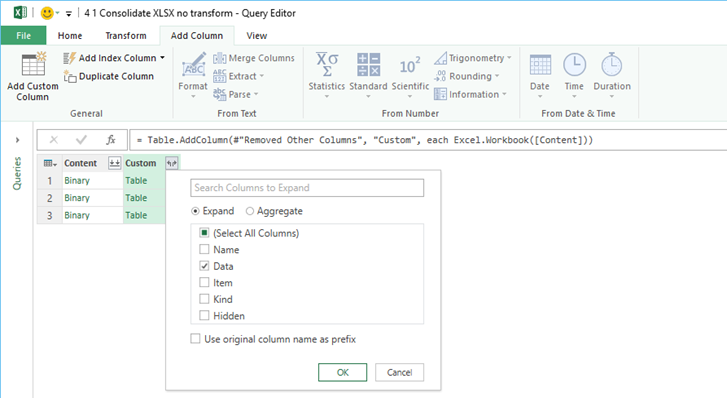
After you add this column, you can then click on the expand button for the new column as shown below.

You will be given a choice of which items to keep from the underlying tables.  You should select the Data option only and deselect the other items in the list.

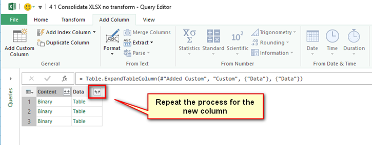
Nothing seems to happen.  You get the window below.  What is happening behind the scenes is that Power Query is working its way through the Excel Object hierarchy to find the underlying data.  Simply click the expand button again.

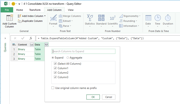
This time keep all the columns and click OK as shown below.

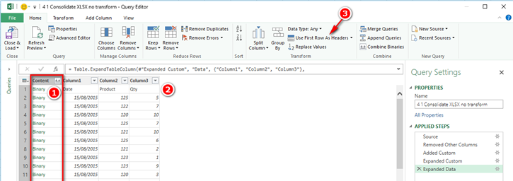
You don’t need the first column any more (shown as 1), so you can remove that (Select the first column and then “Remove Columns”).  Then you will need to promote the first row (shown as 2) to headers by selecting “Use first row as headers” shown as 3 below.

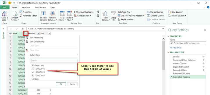
This time when you click one of the filter buttons (shown below) and click “load more”, you will not get an error message (unlike what happened with the CSV example last week).

The reason you don’t get the error is that Power Query has not automatically tried to predict the column data type on your behalf.  Simply deselect the extra header row from the list and click OK.

The last step is to select each column and set the data type manually.  First select the column (1) and from the Home tab (2) change the data type from any (3) to the correct format (4).

You can set more than one column at a time by multi-selecting the columns.

Close and Load, then save the workbook.

A Final Word

The process described in this post is really good when the data is in a tabular format that can be easily combined without transformation. If the file format is not easily combined from its starting format, then it is best to use a function to combine the data as covered in this previous post.

Of course the more files you have to combine (and the greater the frequency of the process) the more benefit you will get (let alone the fact that you are learning new skills).

If you want a comprehensive lesson on how to use Power Query, checkout my training course here https://exceleratorbi.com.au/product/power-query-excel-power-bi-online-training/