Convert a Cell Value into a Column with Power Query

Level: Advanced Power Query

I am in the process of finalising some action items after a great Power BI, Power Pivot and Power Query training course in Melbourne.  During the training we looked at a scenario for one of the attendees where they needed to combine data from multiple Excel files into 1 big table.  I have blogged about this before in 3 articles starting here.

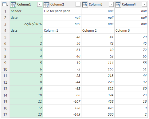
In this specific scenario we looked at in the training, there is a weekly extract of data from another BI system (sound familiar?).  Each week someone must use “Export to Excel” to grab the current week’s data and dump it into a file (a typical action for a BI system that isn’t user friendly).   The file format of the export looks something like this (indicative).

The key points about this data structure are.

1. There is a date in a cell in the file header.
2. The details are also in the same file, but there is no date column in the detail section.

The requirement is to end up with a table like this.

The rest of this article describes how to do it.

Step 1.  Connect to the file using Power Query

Step 2.  Filter the Table so the Date Row is at the Top

To do this, I simply did a “Remove Top Rows” to remove the top 2 rows.

Step 3.  Killer Trick to Extract the Actual Date

The next step is a killer trick.  The idea is to extract the date from the first column in the top row into a scalar value so it can be used later.  To execute this step, you need to use a hand written PQL language formula.

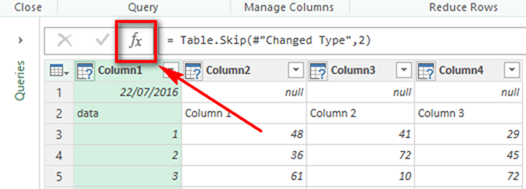
Click on the Fx button to insert a new custom step

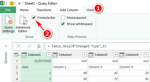
If you can’t see the Fx button, it means you don’t have the formula bar turned on.  Turn it on like this

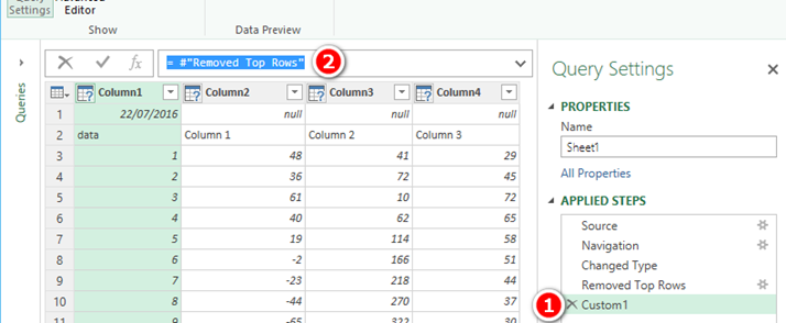
After clicking Fx, a new custom step will be added to the query pane (1 below).  The step (by default) assumes that you want to use the previous step as a starting point (2 below).

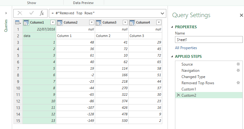
To extract the date as a scalar value (2 below), you need to use the function Record.Field as shown in 1 below.

Note how I have wrapped the original step #”Removed Top Rows” inside the function Record.Field.  The {0} portion of the formula says “take the first row from the previous step, and the “Column1” part says take the data in the column called “Column1”.  The intersection between the first row and this column is a single cell, and hence this formula is accessing the actual value (scalar value) in this one single cell in the workbook.  You can see it is a scalar value (2 above) because it doesn’t show a table, but a single value.

Strictly speaking I didn’t need to force the date into the first row – I just did this because it was cleaner.  I could have just as easily reference the row/column without removing the top rows with this formula

= Record.Field(#”Removed Top Rows”{2},”Column1″)

The number inside the curly braces represents the row number, with a base 0 index.  So 0 is the first row, 1 is the second row etc.

Step 3. Second Killer Trick – Get the Data from an Earlier Step

The next (little known) trick is that I can actually go back and get the data from an earlier step.  Power Query by default always uses the previous step as the starting point for the next step – a logical flow.  But it doesn’t have to be that way.  In this case the previous step is simply the scalar value = date, and that is not what I want. I need the step previous to that which is “Removed Top Rows”. 

Click on the Fx button to create another new custom step.

Now change the formula in the formula bar (1 above) so it points to the step “Removed Top Rows” instead of pointing to the step “Custom1”.  Like this

So now I am back were I was before extracting the Scalar Date value.

Step 4.  Proceed to shape the data the way you want it

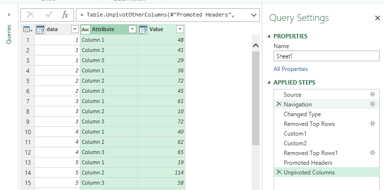
I then executed some steps to cleanse and shape the table the way I want the data.  I ended up with the following.

Step 5.  Add the Date as a Column

The final step is to bring the date from step 2 into a column in the table.  This is quite easy now.

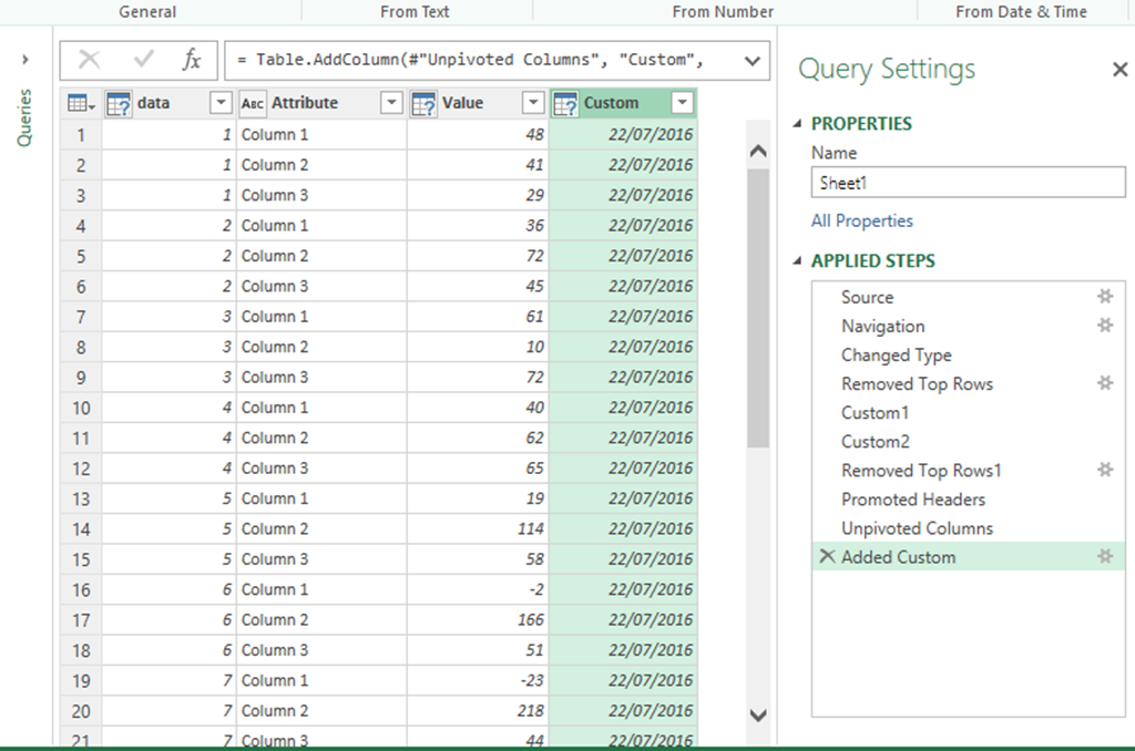
Add a Custom Column, and refer to the step “Custom1” that returned the scalar value

And I end up with this

Exactly the type of data structure needed to load into Power Pivot.  I simply reordered the columns to put the date column first, and then it was done.

Final Comments

If you want to (or need to), you can then turn the above query into a function.  Read more about that here.  If you turn it into a function, you can then use it to process all files in a folder and combine them into a single data table to load to Power Pivot.

If you want to look at the workbook, you can download it here => Extract scalar date