Level: Beginners
When you write a Power Query workbook in Excel 2013, you are given 4 choices of what to do with results. One of the choices is to load the resulting query directly to the Power Pivot data model. This choice does not exist in Excel 2010. It is reasonable therefore to think that you must first send the results to an Excel table and then load the table to Power Pivot, but that is actually not the case – there is a way to do it, read on.
First let’s look at the Excel 2013 UI
You have 4 choices of what to do with your Power Pivot Query in Excel 2013:
- load the results to Power Pivot
- to a table in Excel
- both 1 and 2
- neither 1 or 2
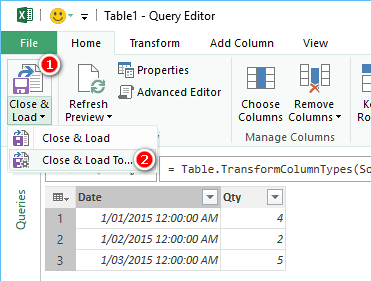
To see the choices, you need to select
- Close and Load
- Close and Load To
You will then see the “Load To” dialog as shown below. The way this dialog is laid out is a bit confusing. At the top of the dialog are 2 radio buttons. You select the first option if you want an Excel table and the second option if you don’t. Then down the bottom is a check box. You “check” the box if you want to load the data to Power Pivot and “uncheck” it if you don’t.
I have no idea why there are 2 different approaches to making these choices, but that’s the way it works. So simply select the combination that you want in order to have 1 of the 4 choices mentioned above.
How to Load to Power Pivot in Excel 2010
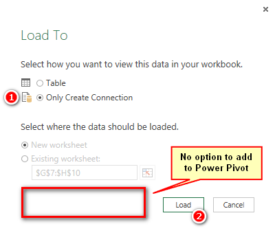
When you click “Close and Load To” in Excel 2010, the dialog box is a bit different. Note that there is no option to send directly to Power Pivot like there was in the Excel 2013 example above.
The best way to add the data from Power Query is to select “Only Create Connection” (shown as #1 above), then click “Load” (shown as #2 above).
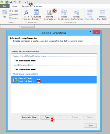
Then go to the Power Pivot window and
- Click on the design menu
- Select Existing Connections
- From the list of workbook connections, select the query you just created
- Click on Open
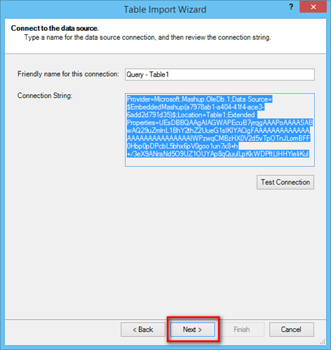
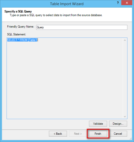
This will open the table import wizard. Click Next.
In the next window, click Finish
And there you have it. Your Power Query results are sent directly into Power Pivot without the need to create an interim table first in Excel.
If you want a comprehensive lesson on how to use Power Query, checkout my training course here https://exceleratorbi.com.au/power-query-online-training/



This is the best explanation I’ve read on the difference between the load options. Thank you- this post has been incredibly helpful for me.
@Oxenskiold and @Matt
A very important thing you must remember in 2010 is once you create the connection you must go to connection properties an on the tab Definition – change Command type to Default instead of SQLalso In command text delete SELET * from [table]
Say OK – This will ensure all columns get imported in the Power Pivot Model
Thanks a lot Sam. Now both the missing columns problem and the refreshing problem are gone.
This actually could have an impact on one of my clients, a small but energetic company with comparatively small computer configurations (especially RAM wise) and computer skills. It’s a long story but the simplicity this solution opens of for will definitely help them.
Thanks to you and also to Matt for posting the blog post.
Thanks for this solution Sam – had been battling with this problem since a few updates ago!
My much more cumbersome solution was to import the table from Workbook Connections, delete the table, then re-import from PowerPivot Data Connections.
With your method I could use VBA to change all Power Query connection types from SQL to Default and delete the command text.
Hi Matt.
I’m a little bit curious as to your experience with this technic. I have tried to use it in the past with a very bad result. Only a few of the fields from the power query table find it’s way into the power pivot table and it’s very difficult to refresh the power pivot table(s) through power query if not impossible.
I’m wondering if there are some steps that I have overlooked?
Well actually I hardly use Excel 2010 in real life scenarios so I am not experienced enough to say. But I would be really surprised if there was inconsistent behaviour. I would expect it either to work in full or not work at all. What might cause it to not work is if you change the power query. Sorry I can’t shed more light
Note that if you modify the Power Query at all then the connection no longer works and you will need to repeat the process and recreate all relationships and measures associated with that table.
Ahh, very good point. Thanks for sharing. I assume you could copy the new connection string from the changed query and replace it, so you don’t have to remove the table. Have you tried that?
Thanks for sharing this valuable resource I already implemented this in Excel.