Cleansing Data with Power Query

Today I am combining a few techniques to show how to build a robust cleansing approach for your data using Power Query.  This article will demonstrate the following Power Query techniques

• Joining tables (Merge Query)
• Self Referencing tables
• Adding Custom Columns

Sample Data

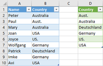
I am using some sample data as shown below.  The Country data is the data I want to cleanse so there are consistent country values in the Country column.

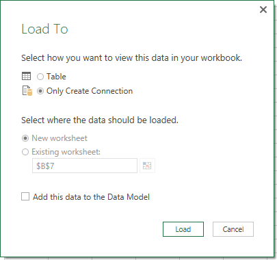
I first load this data into Power Query and set “Close and Load to” so that it only creates a connection.  I then have Power Query access to the source data table that can be reused multiple times.

Create a Table of All Entered Countries

The next step is to produce a list of the unique entries in the source data.  To do this, I referenced the above table by right clicking (1 below), then Reference (2)

I then removed the Name column (1 below) and then removed the duplicates in the remaining Country Column (2 below).

I then sorted the column before loading the data back to Excel as shown below.

Create the Substitutes with a Self Referencing Table

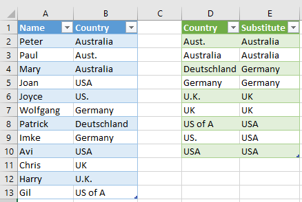
I first covered this trick of a self referencing table in this blog article.  Continuing on with my test data above, I have manually added a new column to the green table above and entered the substitutions as needed.  Where there is no substitute needed I have simply left the substitute blank.

As it currently stands above, if the source table is sorted and then the green table is refreshed, the substitute column will fall out of alignment with the source table – that is bad.  Now for the self referencing trick.  I load this green table above back into Power Query as a new query, setting it to only create a connection as I did for the original set of data. I named this new query “Substitutes”

I then edited the original query that created the original green table and joined it to the substitute table (aka self referencing).  While editing the Entered Names table, I selected Merge Queries (1 below), selected the Substitute table (2), then joined on the Country Columns (3, 4) with a left outer join (5).

I then expanded the new column to extract the substitutes.

This now gives me a self referencing table that will refresh while keeping the countries and substitutes correctly aligned regardless of what happens to the source table.  This is the key point about a self referencing table (covered in my previous article).

Update the New Data

Now when new data is added to the source table, it will appear in the substitute table after refresh as follows.

What would be much better is to be clear which are the correct entries that have previously been checked so it is more obvious which are the new entries.  So I decided to enter the correct country name for each entry as follows.

It is now much clearer that there are 3 new entries that need to be maintained, and I then updated the new data below.

Use the Substitute Table

Now that I have this substitute table working for me, all I need to do is create a new copy of my source table that uses the substitute country rather than the original country entered.  I create a new query referencing my original source data (right click, reference).

Merge the queries as before, joining on the original country column.

expand the table to retrieve the substitute column

Then delete the original country column and rename the substitute column to be called “Country”

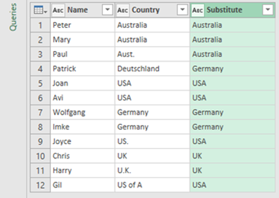
As you can see below, the substitute table is correctly remapping the data as needed.

When the new data is added to the source table, the substitute table will have blank entries as shown below.

As a nice touch, I went back into the final query and added a new custom column as follows

and then used this new column as the country column.  Now when I refresh the data, it is clear that I need to do some maintenance on the substitute table.

If you want a comprehensive lesson on how to use Power Query, checkout my training course here https://exceleratorbi.com.au/product/power-query-excel-power-bi-online-training/