DAX Query Tables in Excel 2010

I was helping a participant at http://powerpivotforum.com.au with a problem. Long story short, she needed to return a table to Excel from a data model – not a Pivot Table. This concept can be a bit strange at first – let me explain.

Tables – Not Pivot Tables

A Pivot Table is a tool that aggregates data and allows you to slice and dice to get different totals and sub totals of that data. This is great when your tables are full of numbers and you want to aggregate those numbers. But consider the following scenario. What if you want to return a table that lists out all the names and addresses of customers that have purchased more than $2,000 in products from your company? Well you could set up a pivot table like this.

In the above Pivot Table, there are 5 different columns from the Customer Table and 1 measure (there are actually many more text columns that I want to extract other than those shown here). The columns of data from the Customer Table have been placed in the rows section of the Pivot Table. The more columns you put on rows in your Pivot Table, the slower the performance will be. What is worse, if the columns come from different tables, you can get an exponential slowdown in performance. Read about why that is here.

OK, so the answer to this problem is don’t use a Pivot Table, but use an Excel Table instead. There are few articles on the web that explain how to do this in Excel 2013 including this one from Scott at TinyLizard.com. I may write my own post about that another time, but today is simply to explain how to do this in Excel 2010 as the process is not the same.

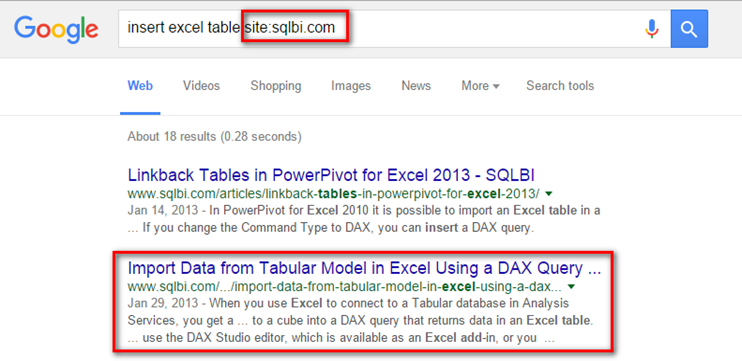
When ever I want to learn something about DAX Queries, I always head over to http://sqlbi.com. A good way to search a specific site is to use the Google SITE: keyword in your search as shown below.

The second item in the list looked promising, so I took a quick read. It refers to inserting tables from a Tabular model, but I thought I could modify the technique for Excel 2010. I did that and it worked – here is the full process.

I have a sample workbook setup using Adventure Works. Here is the data model (shown below) and you can download the workbook here.

1. Click in a blank cell in your workbook
2. Select the Data Menu
3. Click Existing Connections
4. Select PowerPivot Data
5. Click Open
   
6. Select Only Create Connection
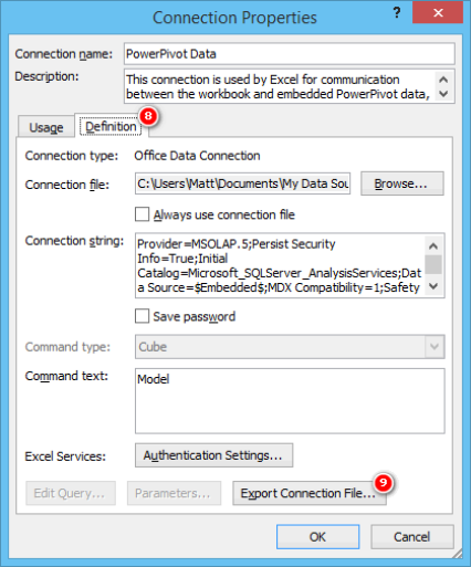
7. Click Properties.
   
8. Click on the Definition Tab
9. Select Export Connection File
   
10. Give your connection a name
11. Click Save
    
12. Open Windows Explorer and browse to the Data Sources folder
13. Right click on your new connection
14. Select Edit in NotePad
    
15. Locate the section of the XML shown in the image below
16. Replace the word Cube with Query
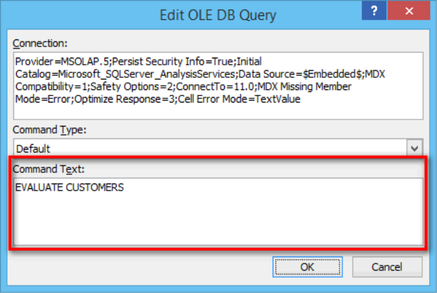
17. Replace the word Model with any valid DAX Query statement. The easiest is simply EVALUATE AnyTableName. I have used EVALUATE CUSTOMERS
    So I started with this
    
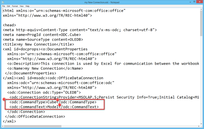
    And ended up with this
    
18. Save and close Notepad.
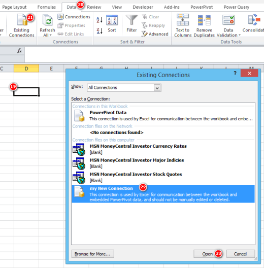
19. Finally, go back to Excel and select a blank cell
20. Navigate to the Data menu
21. Select Existing Connections
22. Select your new connection (from step 10)
23. Click Open
    
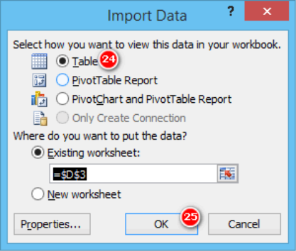
24. You will see the same dialog as in step 4, but this time you have an option to insert a table. Select Table from the list
25. Click OK.
    

And there you have it – a new table in your workbook that is sourced and linked to your data model.

Returning this text detail in a pivot table would not be a pleasant experience.

Now this table is the entire Customers table, and what I really wanted was a list of customers that have purchased > $2,000. To fix that, you will need to write some DAX Query code.

1. Right click anywhere in the table
2. Select Table
3. Select Edit Query

You have the opportunity to replace the query you added in step 17 with any valid DAX Query. I am not going to go into DAX as a Query Language here as that is a topic for another day. To finish off this process, I have added the following DAX Query

EVALUATE
FILTER (
    ADDCOLUMNS ( customers, "Cust Sales", [Total Sales] ),
    [Cust Sales] >= 2000
)

And my table updates with the full list of customers that have sales > $2,000

For more information about writing DAX Queries, I recommend you take a look at this article at SQLBI.com. It is not specifically an intro to DAX queries, but I found it very helpful in learning what can be done.

A Final Word

I am not sure what will happen when others open this workbook. It is unclear to me if the new connection I created is automatically embedded in Excel or if it is still sitting on my PC. I would be interested to hear from any Excel 2010 user that opens the sample workbook to find out if the connection can be edited by them.