Where has Matt been?
 Before teaching you how to pass an Excel parameter to Power Query, I’ll have a few words. Regular readers of my blog may have noticed I have been missing in action over the last month. I have been super busy with the PUG World Tour, delivering a lot of training, finalising my new book Supercharge Power BI, and also taking a couple of weeks vacation.
Side Story: Power BI Training Has Never Been More Popular
I have been delivering Power Pivot/Power BI training for almost 4 years now and the demand has never been greater. My last 5 live training courses in Australia have all had record numbers of participants, and my current semester of live online training (Supercharge Power BI) has 34 active participants. I’m super excited what the future holds for this fantastic product, and it just keeps getting better and better.
Pass an Excel Parameter to Power Query
I was delivering training yesterday in Sydney and one of my students (Stephane) asked me how to pass a parameter from Excel to Power Query. I have written previous articles about this principle and power query filters at PowerPivotPro.com but thought it would be good to blog about how simple it is to do this.
Sample Scenario – Extract Invoices for Selected Date
I am going to demonstrate the concept using the Adventure Works database. In the example below, I have set up a single cell in Excel that contains a date which is then passed to Power Query. When I refresh the query in Excel, the results table is updated with all the orders from the database for the selected date. Note: There are other ways to do this, such as loading all records into Power Pivot and extracting them from there on demand. However there may be people that want to do it this way for what ever reason.
Set up a Parameter Table
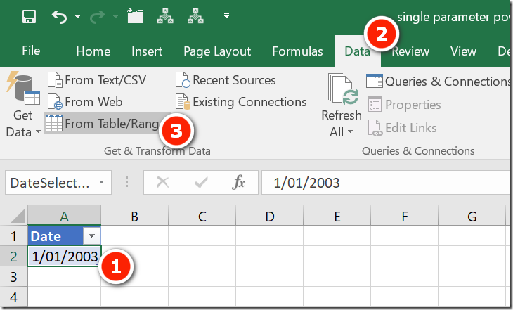
The first thing to do is set up a single cell table that contains the date of the orders to extract. Then click in the cell (1 below), select data (2), from Table/Range (3). Note this is Excel 2016; the UI is slightly different for Excel 2010/2013.
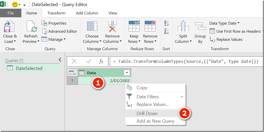
The next step is super simple and is the secret sauce to this process. As you probably realise, the data loaded is a table with a single column and a single row (see below). The table therefore has a single cell that contains a single date. It is not possible to use the date in this tabular format, so it needs to be changed before the date can be used in another query. To do this, simply right click on the cell (1 below) and then select drill down (2).
After completing this step, the table is removed and the actual value is returned by this query (see below).
Now that this is a value (the scalar value shown in 1 above), this query name (2 above) can be directly used inside another query.
Extract the Required Data for a Random Date
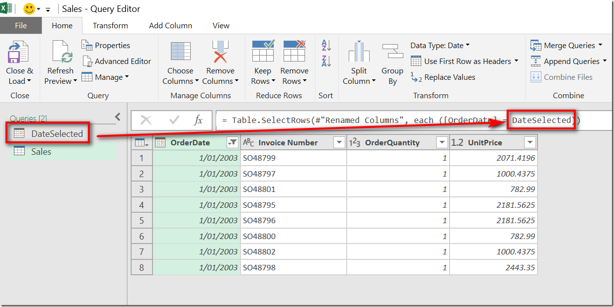
The next thing is to write a query to extract the required data from the database. First set up the query as required, then apply a Power Query filter from the drop down box (1 below) for any random date (2 below).
This creates a query step as shown below – the query step directly references the date selected above. Note: the formula bar needs to be turned on to see this (View\Formula Bar).
It is now very simple. Just manually edit the hard coded date in the code above with the name of the query that returns the date coming from Excel.
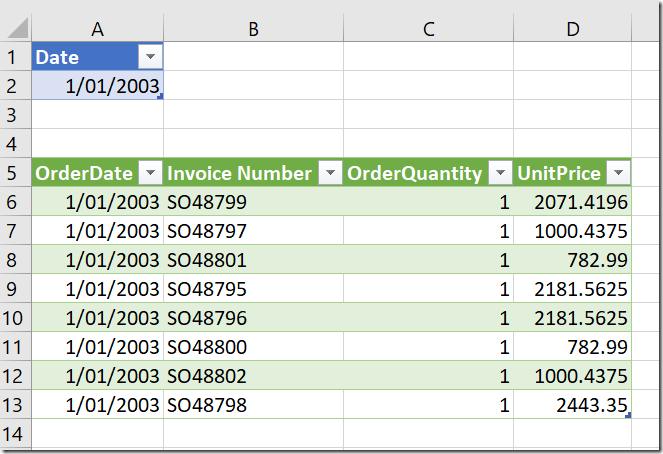
Now close and load. Set the DateSelected query so it doesn’t load and the Sales query so it loads to the original spreadsheet below the date parameter table.
It’s not easy to find how to set a query to not load in Excel after the initial load settings have been configured. Simply right click on the query (in the query pane), select load to, set do not load.
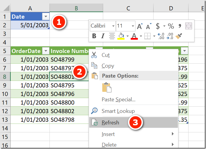
To refresh and extract a different date, simply change the date in the parameter table (1 below), then right click in the results table (2) and then click refresh (3).
The query then runs and the new data is returned to Excel.
A Final Word
This is the most simple parameter table you can create – a single value. Once you understand the principle, you can let your imagination run wild with other things you can do here. If you want to fast track your learning so you can leverage the power of Power Query filters and all about this tool, take a look at my self paced online Power Query training course. This training has over 7 hours of video explaining concepts like this. Once you know how, you will be able to save time and do fantastic things you never dreamed possible.





Question if I may … is there a way to pass a multi value parameter table ie not just a single cell to a Text.StartsWith function?
Wow. Great. So easy.
By manually entering a starting date in my Excel-sheet, I am able to select only the data that has this date as a starting date.
Brilliant, clear instructions, thank you!
Thank you big help and it worked, also created a userform with date dropdown linked to the single cell table with refresh button
Very helpful answer,thanks
Very helpful answer.
Very creative. Well done. Thank you.
Thank you. This was a big help making a query useful to other associates.
Excellent,
Loved this, well explained and its simple. Spend a lot of time on the searching for this solution!
This was the clearest and most helpful explanation I found by a mile. Thanks!
Thank you !!.
This worked well for me, took me a while to match the data type for text and date, but otherwise it pulls in the date from a filename exactly how I wanted to use as a variable in my code. Thank you!
Hi Matt,
This is the easiest way to dynamically parameterize the query.
I had done it using another method in the past. But, really loved the secret sauce.
Thanks a lot.
Nilesh
Do you know how to pass the input variables in excel to Oracle query which is embedded in Excel…?
No idea, sorry.
Matt this is awesome! You should be number one in google search!
Hi Matt,
Can I also pass an Excel parameter to a native query like the one below (on a Progress database)? We are working with big datasets, so I would like to apply the filter before the data is loaded. In this simple example I would like to replace ib240.cdstatus = ‘O’ by ib240.cdstatus = MyParameter.
let
Source = Odbc.Query(“dsn=Extended”, “Select#(lf) ib240.cdorder,#(lf) ib240.cdstatus#(lf)From#(lf) PUB.””ib-240″” ib240#(lf)Where#(lf) ib240.cdstatus = ‘O'”)
in
Source
I guess it depends if the DB accepts parameters or not. You should also investigate Dynamic M Query Parameters (if you are using Power BI) https://docs.microsoft.com/en-us/power-bi/connect-data/desktop-dynamic-m-query-parameters
Thanks for the simple, yet accurate example for using Excel parameters in PQ!
Excellent post, Matt!!
Can you help me with similar request ? I’d appreciate your response
I have a table with this structure
Country City
USA NYC
Canada Toronto
England London
I would like to have the user choose the country from the drop down ( one or many) and then based on the selection , it should display the data.
I was able to write a power query (https://exceleratorbi.com.au/pass-excel-parameter-power-query/ ) but only with one value. Update the value and then hit refresh , the table gets updated.
This is not I am looking for.
What I want is the user to choose one or many values from the dropdown and then those values are passed to the parameter and that filters the table. I tried using similar method using the link above but was unable to find a solution for multiple values.
I’d appreciate if you can provide the steps to create such solution. I am a beginner in Excel Power Query.
Thanks
Danny
Just wanted to say a huge thank you for this, after spending half of the day looking at people advising to invoke functions and copy this code this one post was not only very easy to understand (I’m teaching myself and have only been at it a day) but did exactly what I needed it to do.
Hi Matt.
Thank you for this and got it to work on the one query that only required the date filter. I have another query that also has a from and to date but are used within the query in more ways than just a filter and need to add “Parameters”. The issue I am having is that the date format is the American format 3/31/2018 M/D/YYYY and in SQL the date format I have is 2018-03-31. I tried to use the convert(varchar,@Sdate@,23) but still did not work.
Maybe a way to take your Date table and define it as a Parameter?
Well you can load data from your parameter table and format it any way you need prior to passing it to another query.
I’ve followed all the steps here. But when I click Close & Load, I get an error
“This won’t work because it would move cells in a table on your worksheet”
thoughts?
I’m sorry, I figured that out…but what I haven’t figured out is this
“Set the DateSelected query so it doesn’t load”
I cannot find the setting which tells a query NOT to load to an excel sheet…
It’s not easy to find in Excel after the first load. Right click on the query (in the query pane), select load to, set do not load
You should add this piece to the article. I’ve been scouring google looking for how to do this without any luck. I didn’t think to check these comments…
Hello, thanks for your post. I’m trying to come up with a statement when I need two or more records as criteria. If one record we use {0} in a statement. What if I have two rows I need to use for criteria, i.e. both {0} and {1}. Or bigger range. Thank you so much
Sort the list in the order you want, then use “keep top rows”. You can use this technique for the first row too of course, but you miss out on learning about the M language if you do that.
Thanks a lot for the tutorial!
I would like to filter on the date only if there is a value in the cell, otherwise I’d like not to apply the filter.
How would you do in your example?
Thanks in advance.
Matt, Thanks for the tip. I am using this to filter by processor. The processor picks their name from a drop down box, which is the table that is passed to the power query. I works great. However i would also like to have the full results (see all processors). When i use a blank or All, its reading it as text, and nothing comes back. Is there something that would pull all records? The formula from power query is : Table.SelectRows(#”Added Custom11″, each ([Processor] = RASelect)), with RASelect as the input.
Thanks,
Brett
I’m sure it can be done, but it depends on the query and how it works. I guess it would involve an if statement. If your parameter currently filters a list, then the if should not complete any filter if blank. If the parameter is needed to contain a list of values of the items, you would need to build that list into the query and switch to it in the event the parameter is blank.
I was thinking the same thing. I tried: if RASelect
= null then Table.SelectRows(#”Added Custom11″, each ([Consultant] = RASelect)) else null. I would get an error if RASelect was empty. Is there a function that instructs it to do nothing if null?
To me, the if statement looks fine. There is also a try/otherwise statement that can be used to trap an error. You could look into that.
Instead of null, i just did a sort on the query. It worked. Thanks for the tip and your help.
Excellent tip Matt, let me share my experience trying to use this tip but put the excel cell value as a parameter inside an SQL query.
Hopefully it helps people, since didn’t find so much about this specific usage of PQ parameters.
If excel cell value is a text like Sparepart no problem, the following works:
= Sql.Database(“databaseserver”, “dbname”, [Query=”SELECT * from mytable where Description = “& Dateselected &” “])
If the excel cell value is a date like 20/10/2018, the following doesn’t work:
= Sql.Database(“databaseserver”, “dbname”, [Query=”SELECT * from mytable where Date >= “& Dateselected &” “])
Since SQL expects dates as ’20/10/2018′ I need to convert 20/10/2018 to this format (it took me ages to think about..PQ error messages are crazy….;-)
I didn’t find any direct command in PQ to add the ‘ at the beginning and end of the date, so finallly did the following:
– Created a second column in PQ based on the first one with 20/10/2018, but with an insert at first char, so now have ’20/10/2018
each (Text.Insert(Text.From([firstcolumn]),0,”‘”)
– Created a third column in PQ based on the second one with ’20/10/2018, but with an insert at eleventh char, so now have ’20/10/2018’
each Text.Insert(Text.From([secondcolumn]),11,”‘”)
Once I got the final format, removed the first and the second colum and Drill down and now the SQL query works !!
Don’t know if there is an easier way to convert the date format, I’m PQ beginner, you know?
Thanks
EXACTLY what I was looking for!!!!!!!!!!!
So Easy Peasy.
A cave man (or accountant, same thing) could do it.
Error:
DataSource.Error: Microsoft SQL: Invalid column name ‘Startdate’.
Details:
DataSourceKind=SQL
DataSourcePath=gje-dwht-sql01.gje.osl.basefarm.net\testsql;edw
Message=Invalid column name 'Startdate'.
Number=207
Class=16
SQL:
declare @P1 as int, @P2 as int, @P0 as int
set @P1 = 201801
set @P2 = [Startdate]
set @P0 = 201801
I can’t get this to work with my sql.
Is it perhaps my method of setting the values? (set @P0)
I suggest you ask a question at powerpivotforum with some sample data and an explanation of what you are trying to acheive.
Hi,
I want to pass comma separated values as input to parameter table in Power Query and generate the report. How to do that?
Hi all.
Can we do the same thing but with an vba code?
For instance, I want to select a file and pass that file path to the parameter “File”
Thx
I’m not clear what you are asking.
While I didn’t get a solution from this page that would work for me, the hint from Ivan led me in the right direction. With an Advanced Query (after building a mock up) I came up with the following Power Query language code to query my view X_AllTransactionLines based on a date in the date range:
let
dtmStart = Excel.CurrentWorkbook(){[Name=”rngStartDate”]}[Content]{0}[Column1],
dtmEnd = Excel.CurrentWorkbook(){[Name=”rngEndDate”]}[Content]{0}[Column1],
Source = Sql.Database(“lca07”, “exo_lca_live”, [Query=”select * from X_AllTransactionLines”]),
#”Filtered Rows” = Table.SelectRows(Source, each [TransDate] >= dtmStart and [TransDate] <= dtmEnd)
in
#"Filtered Rows"
I don't mind getting out of a windows UI and into "code", and with it being this easy and understandable I thought I'd share
I’ve used this trick before. However one problem I have (for Excel 2010) is with large tables. The refresh still loads everything and only then filters. It doesn’t let my database do the filtering (which would be faster).
Matt,
When I selected ‘Drill Down’ to convert the ‘Date’ field (and remove the table),
1) Power Query returned formula “= #”Changed Type”[Date]”, not “#”Changed Type”{0}[Date]” as shown; missing the {0} value
2) the parameter did not work when retrieving data
3) After adding the {0} to the formula everything worked as you described
Does changing the date value from a table to a scalar require any special steps to include the {0} in the new formula?
Thank you.
The {0} is a row indicator (zero based). So {0} means the first row, {1} means the second row etc. If you right click on a cell, then drill down, I expect that the {0} will be added (assuming it is the first row). I can’t be sure why you are getting a different experience. Any chance of emailing me a video of what is happening?
I have a function which is part of my standard Library called fGetCellVal
You can use it in Excel to read a named range or in Power BI /Excel to read from a Table
let
fGetCellVal=(tbl as any, optional row as number, optional col as text)=>
// fGetCellVal
let
fGetCellVal=(tbl as any, optional row as number, optional col as text)=>
let
Source = try Excel.CurrentWorkbook(){[Name=tbl]}[Content] otherwise tbl,
rNo = if row = null then 0 else row,
col = if col = null then Record.FieldNames(Source{0}){0} else col,
Value = Record.Field(Source{rNo},col)
in
Value
in
fGetCellVal
Sample usage in Excel : fGetCellVal(“fPath”)
Returns the contents of a Cell named fPath
Sample Usage in Power BI – containing a Table called P having 2 Fields Parameter and Value and having Text “File Path” in the First row under column Parameter and “C:\Data” in column Value
fGetCellVal(P,0,”Value”)
Returns C:\DATA
Matt, another excellent post!
These simple tips are so useful. Keep them coming.
Thanks Matt, it is a very useful technique. In some cases, we don’t even need tables, enough to have NamedRange, let’s say CELLNAME. Then use “shortcut”
= Excel.CurrentWorkbook(){[Name=”CELLNAME”]}[Content]{0}[Column1]
in Power Query to get content of range with name CELLNAME. I use it very often, prefer this method to Parameters, because it is easier to change value in cell than in PQ parameter. Moreover, value in cell can be result of a formula, this adds flexibility.
Ivan, I really like that idea. I guess it is a bit more manual coding so not as accessible to beginners or intermediate people learning the tool, but certainly a great approach that streamlines the source location so it doesn’t have to be a table.
Thanks for this! I found using the normal method of creating a parameter didn’t work because I was getting the error “Query ‘Billing With Descriptions’ (step ‘Grouped Rows’) references other queries or steps, so it may not directly access a data source” which is caused when you try to mix an external query with a local query. (here’s more info about that: https://community.powerbi.com/t5/Desktop/Formula-Firewall-Query-references-other-queries-so-it-may-not/td-p/18619)
I worked around this by adding this line in the Advanced editor to directly get the parameter:
FY=Number.ToText(Excel.CurrentWorkbook(){[Name=”NamedCell”]}[Content]{0}[Column1]),
Also note: Use Number.ToText to use the number in the SQL string.
Hope this helps someone!
Great technique, Matt! I’ve been doing start date and end date in a table, unpivoting them, and then getting the List.Min() and List.Max() as parameters for my date range query.