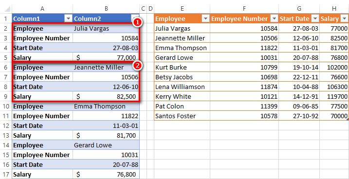
It is very common to need to transform data from one “shape” to another “shape” before it can be used inside Power BI for analysis (although many beginners don’t realise this). One such example is shown below, where the data in the table on the left hand side needs to be transformed into the table on the right hand side. As you can see on the left, column A contains the attribute and column B contains the value of the attribute. Every 4 lines of data is 1 record. This specific problem is very common problem when your only source of data is from an extract (eg csv) from some other system, particularly older systems where you can’t change the format of the data extract.

The trick to solving this problem is to pivot the text data into a tabular shape. I learnt how to solve this problem from my friend Imke Feldmann at The BIcountant.
You Cannot Pivot Text Data Directly
This is how NOT to do it. If you click on column A above and select “Pivot Column” from Power Query, you will get the results shown below.

This approach will not solve this problem because Power Query doesn’t know how to uniquely identify each record set, and that is a hint on how to solve this problem.
How to Pivot Text Data
The trick to solve this problem is to first stamp each set of 4 rows as a unique record.
In the example above, each record is spread over 4 consecutive rows in the table, so we first need to stamp a unique record number ID to each set of 4 rows that makes up a single record. Once we have this unique identifier for each row, we can use the identifier to pivot the data to produce the desired results.
Steps for Pivoting Text Data
I completed the demo below using Power Query for Excel, but of course it also applies to Power Query for Power BI. You can download the sample workbook here.
Step 1:
I loaded the table into Power Query, selecting Data tab (see 1 below) and then clicking on From Table/Range (see 2 below).

Step 2:
In the Power Query window, I went to the Add Column tab (see 1 below) and clicked on Index Column (see 2 below). A new numeric column is added (see 3 below).

Step 3:
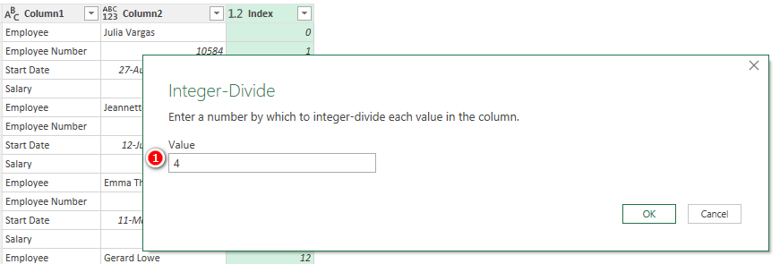
Next, I converted this numeric column so that it identifies (stamps) each record uniquely. For this I went to Transform tab (see 1 below), Standard (see 2 below) and clicked Integer-Divide (see 3 below).

I divided by 4 (see 1 below) as that is the number of rows in each record.

There is now a unique integer in the new column that identifies each record (see 0, 1, 2, 3, 4, 5 below) in the table.

Step 4: This is the final step.
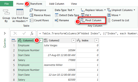
I selected the first column (see 1 below), went to Transform tab (see 2 below) and then selected Pivot Column (see 3 below).

In the Pivot Column dialog box (see 1 below) I selected the Values Column to be Column2 (see 2 below) and then selected Advanced Options (see 3 below) and set to Don’t Aggregate (see 4
below)
.
This pivoted the data as shown below.

I do not need the index column anymore and I deleted it. I then fixed the data formats, and that’s it.

Once I load this table back into Excel beside the original table, it looks as in the first image that we started with in this article.
What Next?
If you want a comprehensive lesson on how to use Power Query, checkout my training course here https://xbi.com.au/pqt
You can learn similar tricks and tips to this on Power Query with illustrative examples. All the examples demoed in the course are also available to download in the course material so that you can practice along as you view the videos for an in-depth understanding of the concepts.


ehodeaysiepufmoumspchajzihdtkl
Great UI solution.
for the M code solution I think the below code would be an option:
= Table.Combine( List.Transform( Table.Split( Source,4),each Table.PromoteHeaders(Table.Transpose(_))),type table [Employee=text,Employee Number=number,Start Date=date,Salary=Currency.Type])
I used the second argument of Table.Combine function based on a recent post by Rick de Groot in this link : https://www.linkedin.com/feed/update/urn:li:activity:7149415015266074624?updateEntityUrn=urn%3Ali%3Afs_feedUpdate%3A%28V2%2Curn%3Ali%3Aactivity%3A7149415015266074624%29
You’re a champion.. i spent much longer than i hope to reveal tryinfg to solve this. Thanks for the solution
Hi, thats a nice trick.
It might be even easier though, if click “Pivot Column”, then in the pop-up windows open “advanced options” and select “Don’t aggregate” in the dropdown. Then you will get the text values directly. (just need to choose the value columns you need)
Hi Matt,
If I’ve understood this correctly then it only works when you have a defined record structure. For example if your Employee’s had multiple Employee Numbers then you get an error. I have groups of payment sub-categories that appear under multiple categories and am trying to pivot those into a tabular structure. I’ll keep searching, but thought it worth mentioning what appears to me to be a limitation with the method above.
Any ideas on solving this would be appreciated.
Thanks for a helpful website.
Yes, this approach is for a regular repeating pattern. You would need a way to identify the rows belonging to a single record and then number them uniquely. You could take a look at this article by Ken Puls, and or consider taking the Power Query Academy course at Skilwave.training.
Hey Matt,
nice walkthrough I had to use similar steps at a project for my client. However the performance reaaaaally slows down once this whole table got to a few million rows and to me it seems that Power BI can´t handle pivoting really large datasets.
Do you have any suggestion how to improve the performance in this matter? I have reduced all necessary columns, I split the date and time columns and tried to avoid any unnecessary steps.
The solution I came up with so far is to split the data per month and then merge it together since pivoting data is working flawlessly when the dataset is small, but once it gets bigger the reload time takes a long time (5min+).
I´d love to hear any tips!
Best regards,
Nico
I wish I had an answer, but sorry – no. Actually, I think 5 mins is not too bad. All I can suggest is to
1. Create a queue of new files to be processed (assuming it is more than 1 file).
2. Run the queue once and export the entire table (transposed) to a history file.
3. remove those files that were processed from the queue to an archive
4. Load the history file as a “history” file
5. Add the new files to the queue and process (a small queue).
6. Append the history file to the new data.
I use this process a lot when Power Query slows down after the quantity of data gets too large.